Case study: Partial profiles

First, the library is loaded:

library(malan)

For reproducibility, the seed for the (pseudo) random number generator is set:

set.seed(1)

Population simulation

First, the population sizes are determined:

population_sizes <- round(c(rep(100, 10), 100*1.02^(1:10)))
plot(population_sizes, type = "b")

A population can be simulated (hiding progress information) as follows:

set.seed(1) # For reproducibility
sim_res_growth <- sample_geneology_varying_size(
  population_sizes = population_sizes, 
  
  # VRS = 0.2:
  enable_gamma_variance_extension = TRUE,
  gamma_parameter_shape = 5,
  gamma_parameter_scale = 1/5,
  
  # Live population: 
  # 3 generations
  generations_full = 3, 
  generations_return = 3,
  
  progress = FALSE)

Live population:

live_pop <- sim_res_growth$individuals_generations

Building the pedigrees

Until pedigrees are build/infered, there is not much information available (e.g. about children). So let us infer the pedigrees:

pedigrees <- build_pedigrees(sim_res_growth$population, progress = FALSE)
pedigrees

## List of 11 pedigrees (of size 217, 96, 95, 56, 51, 47, ...)

pedigrees_count(pedigrees)

## [1] 11

pedigrees_table(pedigrees)

##  33  37  39  21  47  38  51  56  95  96 217 
##   1   1   1   1   1   1   1   1   1   1   1

pedigree_size(pedigrees[[1]])

## [1] 217

We can look at the population as a (tidy)graph:

g <- as_tbl_graph(pedigrees)
g

## # A tbl_graph: 730 nodes and 719 edges
## #
## # A rooted forest with 11 trees
## #
## # A tibble: 730 × 4
##   name  gens_from_final ped_id haplotype
##   <chr>           <int>  <int> <list>   
## 1 727                19      4 <int [0]>
## 2 713                18      4 <int [0]>
## 3 704                17      4 <int [0]>
## 4 688                16      4 <int [0]>
## 5 685                15      4 <int [0]>
## 6 673                14      4 <int [0]>
## # ℹ 724 more rows
## #
## # A tibble: 719 × 2
##    from    to
##   <int> <int>
## 1     1     2
## 2     2     3
## 3     3     4
## # ℹ 716 more rows

This can be plotted:

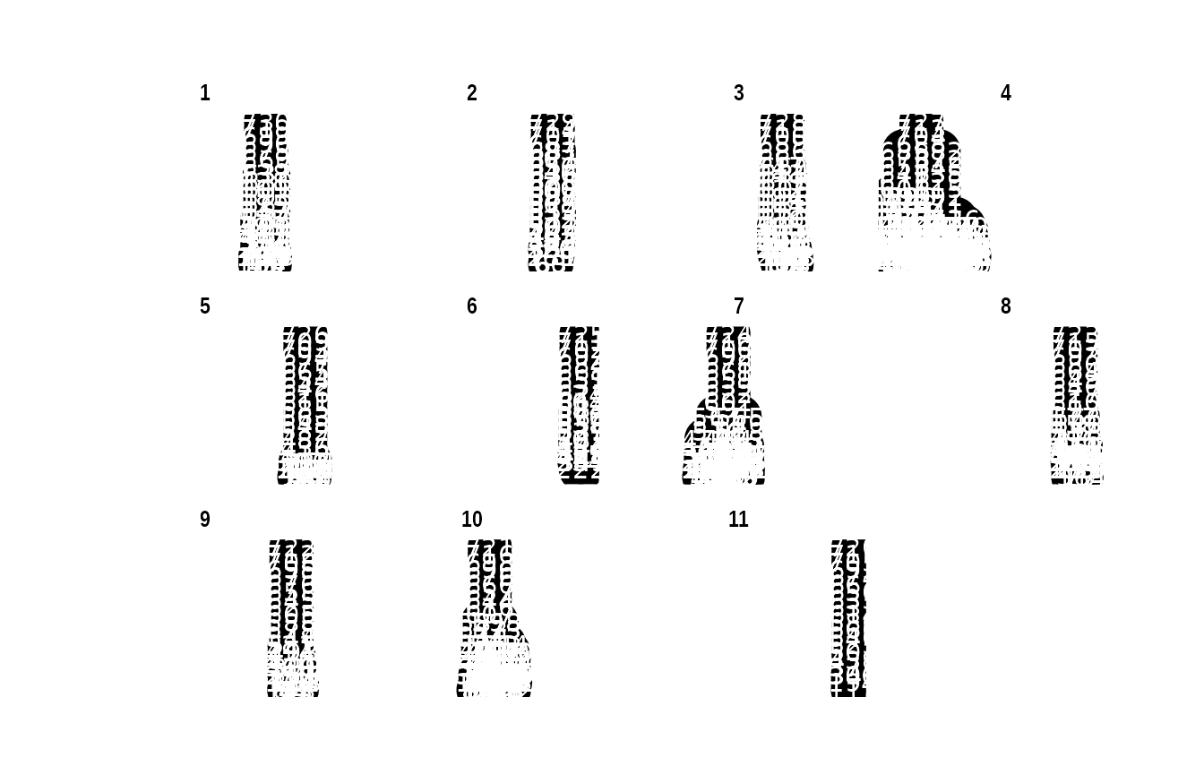
if (requireNamespace("ggraph", quietly = TRUE)) {
  library(ggraph)
  p <- ggraph(g, layout = 'tree') +
    geom_edge_link() +
    geom_node_point(size = 8) +
    geom_node_text(aes(label = name), color = "white") +
    facet_nodes(~ ped_id) +
    theme_graph() 
  
  print(p)
}

## Loading required package: ggplot2

## Warning: Using the `size` aesthetic in this geom was deprecated in ggplot2 3.4.0.
## ℹ Please use `linewidth` in the `default_aes` field and elsewhere instead.
## This warning is displayed once every 8 hours.
## Call `lifecycle::last_lifecycle_warnings()` to see where this warning was
## generated.

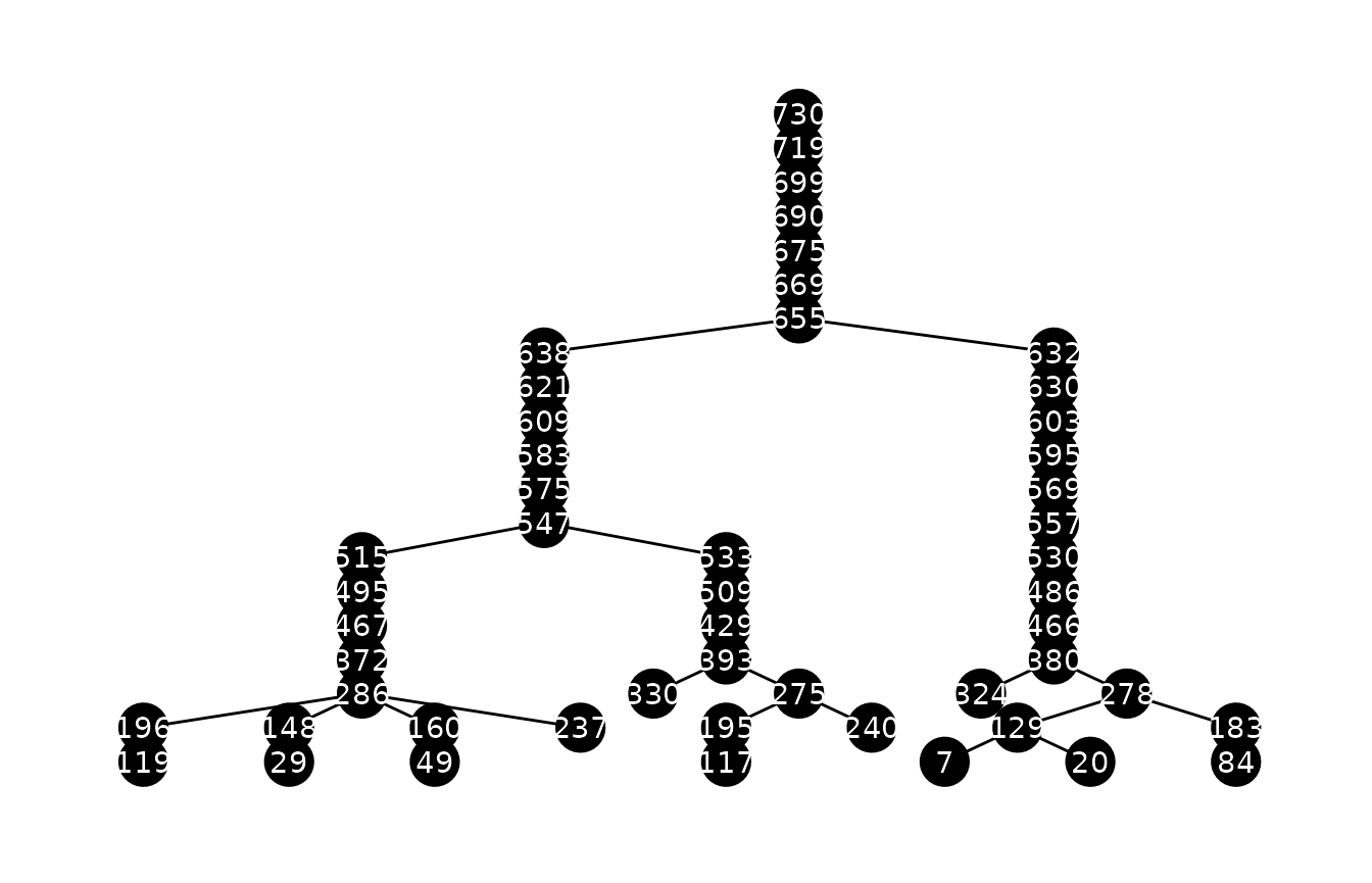
This is rather difficult to make any sense of. Let’s instead plot only pedigree 1:

PED_ID <- 1

g_ped2 <- g %>% 
  activate(nodes) %>% 
  filter(ped_id == PED_ID)

if (requireNamespace("ggraph", quietly = TRUE)) {
  library(ggraph)
  p <- ggraph(g_ped2, layout = 'tree') +
      geom_edge_link() +
      geom_node_point(size = 8) +
      geom_node_text(aes(label = name), color = "white") +
      theme_graph() 
  print(p)
}

Run a mutation process

Up until now, only the genealogy has been simulated. Now, we run a mutational process, i.e. assign haplotypes to founders and let haplotypes flow down the individuals.

We use realistic data. In the package, there is information about the individual markers:

ystr_markers

## # A tibble: 29 × 5
##    Marker  Mutations Meioses  MutProb Alleles   
##    <fct>       <dbl>   <dbl>    <dbl> <list>    
##  1 DYS438          4   10673 0.000375 <dbl [22]>
##  2 DYS392          8   15418 0.000519 <dbl [22]>
##  3 DYS393         15   14264 0.00105  <dbl [17]>
##  4 DYS437         13   10652 0.00122  <dbl [15]>
##  5 DYS385a        32   26171 0.00122  <dbl [52]>
##  6 DYS385b        32   26171 0.00122  <dbl [52]>
##  7 DYS643          3    2220 0.00135  <dbl [17]>
##  8 DYS448         11    7229 0.00152  <dbl [36]>
##  9 DYS390         33   15612 0.00211  <dbl [19]>
## 10 DYS19          36   16090 0.00224  <dbl [19]>
## # ℹ 19 more rows

Note, that MutProb is the point estimate given by MutProb = Mutations / Meioses. Information about which markers that are in which kit is also provided:

ystr_kits

## # A tibble: 88 × 2
##    Marker   Kit        
##    <fct>    <fct>      
##  1 DYS392   Minimal    
##  2 DYS393   Minimal    
##  3 DYS385a  Minimal    
##  4 DYS385b  Minimal    
##  5 DYS390   Minimal    
##  6 DYS19    Minimal    
##  7 DYS391   Minimal    
##  8 DYS389I  Minimal    
##  9 DYS389II Minimal    
## 10 DYS438   PowerPlex Y
## # ℹ 78 more rows

ystr_kits %>% count(Kit)

## # A tibble: 5 × 2
##   Kit               n
##   <fct>         <int>
## 1 Minimal           9
## 2 PowerPlex Y      12
## 3 Yfiler           17
## 4 PowerPlex Y23    23
## 5 Yfiler Plus      27

Let us take all PowerPlex Y23 markers and assume that we only have a partial profile where DYS437 and DYS448 dropped out. At the same time, we also filter out the integer alleles (for generating random founder haplotypes in a minute):

partial_kit <- ystr_kits %>% 
  filter(Kit == "PowerPlex Y23") %>% 
  inner_join(ystr_markers, by = "Marker") %>% 
  filter(!(Marker %in% c("DYS437", "DYS448"))) %>% 
  rowwise() %>% # To work on each row
  mutate(IntegerAlleles = list(Alleles[Alleles == round(Alleles)]),
         MinIntAllele = min(IntegerAlleles),
         MaxIntAllele = max(IntegerAlleles)) %>% 
  ungroup() %>% 
  select(-Kit, -Alleles)
partial_kit

## # A tibble: 21 × 7
##    Marker  Mutations Meioses  MutProb IntegerAlleles MinIntAllele MaxIntAllele
##    <fct>       <dbl>   <dbl>    <dbl> <list>                <dbl>        <dbl>
##  1 DYS438          4   10673 0.000375 <dbl [14]>                5           19
##  2 DYS392          8   15418 0.000519 <dbl [14]>                6           20
##  3 DYS393         15   14264 0.00105  <dbl [12]>                7           18
##  4 DYS385a        32   26171 0.00122  <dbl [23]>                6           28
##  5 DYS385b        32   26171 0.00122  <dbl [23]>                6           28
##  6 DYS643          3    2220 0.00135  <dbl [13]>                4           17
##  7 DYS390         33   15612 0.00211  <dbl [14]>               17           30
##  8 DYS19          36   16090 0.00224  <dbl [12]>                9           20
##  9 DYS391         38   15486 0.00245  <dbl [12]>                5           16
## 10 DYS389I        42   14339 0.00293  <dbl [9]>                 9           17
## # ℹ 11 more rows

This “partial kit” has the following mutation probabilities:

mu <- partial_kit %>% pull(MutProb)
mu

##  [1] 0.0003747775 0.0005188740 0.0010515984 0.0012227274 0.0012227274
##  [6] 0.0013513514 0.0021137586 0.0022374145 0.0024538293 0.0029290746
## [11] 0.0030266344 0.0036747818 0.0037541061 0.0041229909 0.0042882833
## [16] 0.0043338286 0.0050205386 0.0054475439 0.0063641395 0.0133475707
## [21] 0.0147194112

We can make a founder haplotype generator as follows (sampling alleles randomly is not how Y-STR works, but it may work fine for founder haplotypes):

generate_random_haplotype <- function() {
  partial_kit %>% 
    rowwise() %>% 
    mutate(Allele = IntegerAlleles[sample.int(length(IntegerAlleles), 1)]) %>% 
    pull(Allele)
}

Now, a new haplotype is created everytime the function is called (with no arguments):

generate_random_haplotype()

##  [1] 11 14 16 14  6 17 26 16 10 13 20 13  9 28 14 27 31 13 18 24 22

generate_random_haplotype()

##  [1] 18 17 18 14 28 13 30 17 12 11 18  8 11 33 12 17 16 11 17 19 13

Of course such generator can also be created for a reference database with Y-STR profiles.

Now, we are ready to assign haplotypes to the genealogy:

set.seed(1)
pedigrees_all_populate_haplotypes_custom_founders(
  pedigrees = pedigrees, 
  get_founder_haplotype = generate_random_haplotype,
  mutation_rates = mu,
  progress = FALSE)

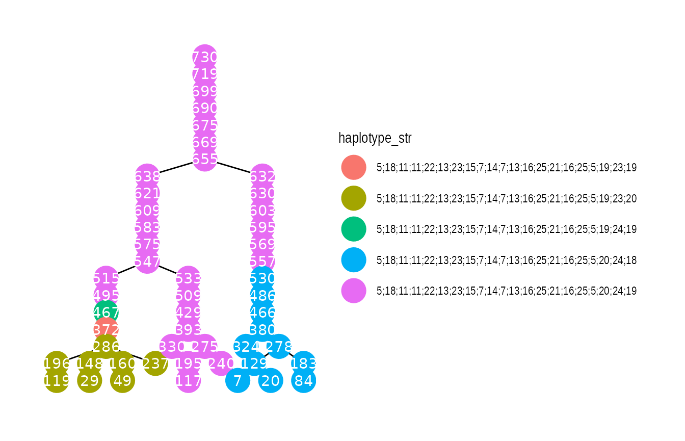
We can now plot pedigrees with haplotype information (note that as_tbl_graph needs to be called again):

g_ped2 <- as_tbl_graph(pedigrees) %>% 
  activate(nodes) %>% 
  filter(ped_id == PED_ID) %>%
  group_by(name) %>% 
  mutate(haplotype_str = paste0(haplotype[[1]], collapse = ";"))
  #mutate(haplotype_str = map(haplotype, paste0, collapse = ";")[[1]])

if (requireNamespace("ggraph", quietly = TRUE)) {
  library(ggraph)
  p <- ggraph(g_ped2, layout = 'tree') +
      geom_edge_link() +
      geom_node_point(aes(color = haplotype_str), size = 8) +
      geom_node_text(aes(label = name), color = "white") +
      theme_graph() 
  print(p)
}

Counting matches

We have live_pop from the population.

Drawing an individual and counting matches

set.seed(5)
Q_index <- sample.int(n = length(live_pop), size = 1)
Q <- live_pop[[Q_index]]
print_individual(Q)

##   pid = 322 with father pid = 376 and no children

Q_hap <- get_haplotype(Q)
Q_hap

##  [1] 13  9 13  6  7 17 23 19  6 11  6 11  9 32 14 28 25 11 18 24 14

Now, count matches in live part of pedigree and in live part of population:

Q_ped <- get_pedigree_from_individual(Q)
ped_live_matches <- count_haplotype_occurrences_pedigree(
  pedigree = Q_ped, 
  haplotype = Q_hap, 
  generation_upper_bound_in_result = 2) # gen 0, 1, 2
pop_live_matches <- count_haplotype_occurrences_individuals(
  individuals = live_pop, 
  haplotype = Q_hap)

ped_live_matches

## [1] 36

pop_live_matches

## [1] 36

We can also inspect pedigree matches information about number of meioses and \(L_1\) distances:

path_details <- pedigree_haplotype_matches_in_pedigree_meiosis_L1_dists(
  suspect = Q, 
  generation_upper_bound_in_result = 2)

nrow(path_details)

## [1] 36

head(path_details)

##      meioses max_L1 pid
## [1,]      16      0 319
## [2,]      16      0 339
## [3,]      16      0 289
## [4,]      17      0 157
## [5,]      18      0  45
## [6,]      17      0 177

This can of course be repeated to many populations (genealogies, haplotype processes, suspects etc.). Also note that variability can be put on mutation rates, e.g. by a Bayesian approach.

Mikkel Meyer Andersen

28 november, 2023

Population simulation

Building the pedigrees

Run a mutation process

Counting matches

Drawing an individual and counting matches