library(snpbeadchip)
library(data.table)
library(mclust)
#> Package 'mclust' version 5.4.10
#> Type 'citation("mclust")' for citing this R package in publications.
library(ggplot2)
Load data
Can use illuminaio::readIDAT() directly, or use this
package’s function read_idat_single().
Here is a skeleton:
library(data.table)
library(omni54manifest)

idat <- read_idat_single("/path/to/files/", "001_Red.idat", "002_Grn.idat")
setnames(idat, "Name", "Address_ID")

manifest <- load_manifest() # From omni54manifest
m_idat <- annotate_manifest_with_idat(manifest, idat)
m_idat
You end up with something like the included example dataset (which is just simulated data):
data(idat_ex, package = "snpbeadchip")
data(idat_ex)
colnames(idat_ex)
#>  [1] "Name"                   "IlmnID"                 "RsID"
#>  [4] "Chr"                    "MapInfo"                "AddressA_ID"
#>  [7] "AddressB_ID"            "GenomeBuild"            "SNP"
#> [10] "IlmnStrand"             "SourceStrand"           "TopGenomicSeqSBE"
#> [13] "TopGenomicSeqSBE_Left"  "TopGenomicSeqSBE_Right" "BeadSetID"
#> [16] "Exp_Clusters"           "RefStrand"              "ProbeType"
#> [19] "SNPType"                "Exclude"                "MappingComment"
#> [22] "A_Red_Mean"             "A_Grn_Mean"             "B_Red_Mean"
#> [25] "B_Grn_Mean"             "A_Red_SD"               "A_Grn_SD"
#> [28] "B_Red_SD"               "B_Grn_SD"               "A_Red_NBeads"
#> [31] "A_Grn_NBeads"           "B_Red_NBeads"           "B_Grn_NBeads"
dim(idat_ex)
#> [1] 200  33
head(idat_ex)
#>          Name                                        IlmnID       RsID Chr
#> 1: rs10000911 IlmnSeq_rs10000911_IlmnDup-131_B_F_2336897696 rs10000911   4
#> 2: rs10000988 IlmnSeq_rs10000988_IlmnDup-131_B_F_2336897694 rs10000988   4
#> 3: rs10002181 IlmnSeq_rs10002181_IlmnDup-131_T_F_2336897690 rs10002181   4
#> 4: rs10005140 IlmnSeq_rs10005140_IlmnDup-131_T_F_2336897678 rs10005140   4
#> 5: rs10005242 IlmnSeq_rs10005242_IlmnDup-131_T_F_2336897676 rs10005242   4
#> 6: rs10010434 IlmnSeq_rs10010434_IlmnDup-131_B_R_2336897669 rs10010434   4
#>      MapInfo AddressA_ID AddressB_ID GenomeBuild   SNP IlmnStrand SourceStrand
#> 1: 143215040    31722985          NA          38 [T/G]        BOT          BOT
#> 2:  75085045    27622566          NA          38 [T/C]        BOT          BOT
#> 3: 141329261    75688121          NA          38 [A/G]        TOP          TOP
#> 4:  22363980    78784850          NA          38 [A/G]        TOP          TOP
#> 5:   5947831    68775897          NA          38 [A/G]        TOP          TOP
#> 6:   2699813    83689289          NA          38 [T/C]        BOT          TOP
#>    TopGenomicSeqSBE TopGenomicSeqSBE_Left TopGenomicSeqSBE_Right BeadSetID
#> 1:          T[A/C]A                     T                      A      1288
#> 2:          C[A/G]T                     C                      T      1288
#> 3:          C[A/G]A                     C                      A      1288
#> 4:          A[A/G]t                     A                      t      1288
#> 5:          T[A/G]C                     T                      C      1288
#> 6:          C[A/G]G                     C                      G      1288
#>    Exp_Clusters RefStrand ProbeType SNPType Exclude MappingComment A_Red_Mean
#> 1:            3         +        II   UNAMB   FALSE                      1006
#> 2:            3         +        II   UNAMB   FALSE                      1522
#> 3:            3         +        II   UNAMB   FALSE                       854
#> 4:            3         +        II   UNAMB   FALSE                       809
#> 5:            3         +        II   UNAMB   FALSE                      7147
#> 6:            3         -        II   UNAMB   FALSE                       857
#>    A_Grn_Mean B_Red_Mean B_Grn_Mean A_Red_SD A_Grn_SD B_Red_SD B_Grn_SD
#> 1:        715         NA         NA      285      472       NA       NA
#> 2:      24282         NA         NA     2051      629       NA       NA
#> 3:      21942         NA         NA      677      524       NA       NA
#> 4:        360         NA         NA      739      536       NA       NA
#> 5:      13063         NA         NA      568      298       NA       NA
#> 6:       1641         NA         NA      302      485       NA       NA
#>    A_Red_NBeads A_Grn_NBeads B_Red_NBeads B_Grn_NBeads
#> 1:           32            6           NA           NA
#> 2:           11           17           NA           NA
#> 3:           12           10           NA           NA
#> 4:           18           15           NA           NA
#> 5:           14           13           NA           NA
#> 6:           12           13           NA           NA
Bookkeeping
The function channel_probe_to_alleles() is used to
select the right addresses and colour channels to easier get mean signal
intensity for allele A and B:
d <- cbind(idat_ex, channel_probe_to_alleles(idat_ex))
d$SNP1 <- substr(d$SNP, 2, 2)
d$SNP2 <- substr(d$SNP, 4, 4)
d <- d[, c("RsID", "SNP1", "SNP2", "RefStrand", "Allele_A_sig_Mean", "Allele_B_sig_Mean")]

d_trans <- data.table(x = log(d$Allele_A_sig_Mean + 1),
                      y = log(d$Allele_B_sig_Mean + 1))
Call alleles
Either train own model like (not easy with this small dataset)
Or use the supplied one:
fit <- get_call_model() Then call alleles:
pred <- predict(fit, newdata = d_trans)
grp <- apply(pred$z, 1, which.max)
prb <- apply(pred$z, 1, max)
Convert clusters to alleles:
grp_AB <- cluster_to_AB(grp)
grp_PM <- to_plus_minus(grp_AB, d$SNP1, d$SNP2, d$RefStrand, sep = "")
table(grp_AB)
#> grp_AB
#> AB BB AA
#> 79 65 56
table(grp_PM)
#> grp_PM
#> AG AT CC CG GC GG TA TC TG TT AA
#> 25  7 34  9 12 42  7 15  4 22 23
table(grp_AB, grp_PM)
#>       grp_PM
#> grp_AB AG AT CC CG GC GG TA TC TG TT AA
#>     AB 25  7  0  9 12  0  7 15  4  0  0
#>     BB  0  0 25  0  0 31  0  0  0  6  3
#>     AA  0  0  9  0  0 11  0  0  0 16 20
Want to impose a threshold?
grp_PM_NC <- ifelse(prb < 0.99, "NC", grp_PM)
sum(grp_PM_NC == "NC")
#> [1] 15
mean(grp_PM_NC == "NC")
#> [1] 0.075
table(grp_PM_NC)
#> grp_PM_NC
#> AG AT CC CG GC GG NC TA TC TG TT AA
#> 24  6 33  9 11 38 15  5 13  3 20 23
Inspect information for certain posterior probability:
d_pred <- d
d_pred$prob <- prb
d_pred$PM <- grp_PM
d_pred[prob < 0.8, ]
#>          RsID SNP1 SNP2 RefStrand Allele_A_sig_Mean Allele_B_sig_Mean      prob
#> 1: rs10114570    T    C         +              5846              1368 0.7804533
#> 2:  rs3817687    C    G         -              9884             17810 0.7817826
#> 3:  rs6670616    A    T         -              5133              1279 0.5769653
#>    PM
#> 1: TT
#> 2: CC
#> 3: TA

idat_ex_pred <- idat_ex
idat_ex_pred$prob <- prb
idat_ex_pred$PM <- grp_PM
idat_ex_pred[prob < 0.8, ]
#>          Name                                        IlmnID       RsID Chr
#> 1: rs10114570 IlmnSeq_rs10114570_IlmnDup-131_B_F_2336897509 rs10114570   9
#> 2:  rs3817687  IlmnSeq_rs3817687_IlmnDup-131_T_R_2336873167  rs3817687   8
#> 3:  rs6670616  IlmnSeq_rs6670616_IlmnDup-131_T_R_2336876340  rs6670616   1
#>      MapInfo AddressA_ID AddressB_ID GenomeBuild   SNP IlmnStrand SourceStrand
#> 1:  25830484    29808538          NA          38 [T/C]        BOT          BOT
#> 2: 138145481    79609986    29657907          38 [C/G]        TOP          BOT
#> 3:  70929200    65709915     7734111          38 [A/T]        TOP          BOT
#>    TopGenomicSeqSBE TopGenomicSeqSBE_Left TopGenomicSeqSBE_Right BeadSetID
#> 1:          C[A/G]T                     C                      T      1288
#> 2:          A[C/G]C                     A                      C      1288
#> 3:          A[A/T]A                     A                      A      1288
#>    Exp_Clusters RefStrand ProbeType SNPType Exclude MappingComment A_Red_Mean
#> 1:            3         +        II   UNAMB   FALSE                      5846
#> 2:            3         -         I     AMB   FALSE                     11190
#> 3:            3         -         I     AMB   FALSE                      5133
#>    A_Grn_Mean B_Red_Mean B_Grn_Mean A_Red_SD A_Grn_SD B_Red_SD B_Grn_SD
#> 1:       1368         NA         NA      536      760       NA       NA
#> 2:       9884       6422      17810      511      536      338      171
#> 3:       3306       1279       1474     1370     1006      692     2040
#>    A_Red_NBeads A_Grn_NBeads B_Red_NBeads B_Grn_NBeads      prob PM
#> 1:            9           12           NA           NA 0.7804533 TT
#> 2:           18           13           12           21 0.7817826 CC
#> 3:           19           27            9            9 0.5769653 TA
Visualisation
alpha <- 0.9
elipses <- do.call(rbind, lapply(seq_len(fit$G), function(j) {

    mu <- fit$parameters$mean[, j]
    S <- fit$parameters$variance$sigma[,,j]

    mat <- mixtools::ellipse(mu = mu, sigma = S,
                               alpha = 1 - alpha,
                               npoints = 250,
                               newplot = FALSE,
                               draw = FALSE)
    colnames(mat) <- c("x", "y")
    mat <- as.data.frame(mat)
    mat$grp <- c("BB", "AB", "AA")[j]
    mat
}))
ggplot(d_pred, aes(log(Allele_A_sig_Mean + 1),
                   log(Allele_B_sig_Mean + 1))) +
  geom_hex() +
  geom_path(aes(x = x, y = y, group = grp, color = grp),
size = 1, alpha = 1, data = elipses) 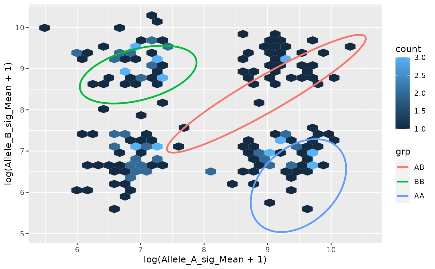
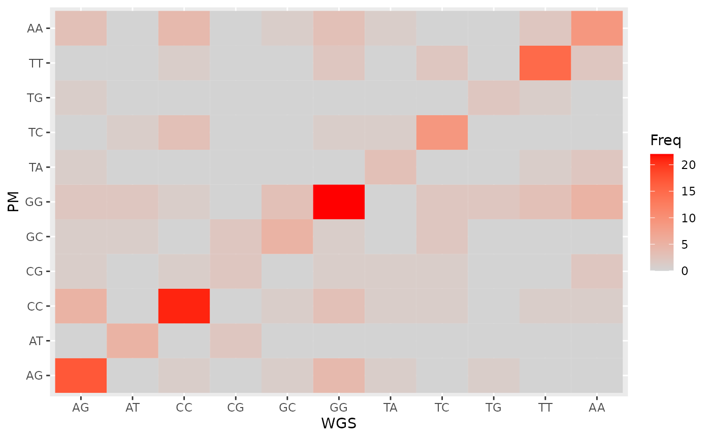
Concordance
We imagine we had the whole-genome sequencing result:
set.seed(1)
d_pred$WGS <- d_pred$PM
d_pred$WGS[sample(seq_along(d_pred$WGS), 100)] <- d_pred$WGS[sample(seq_along(d_pred$WGS), 100)]

d_pred_tmp <- as.data.frame(xtabs(~ WGS + PM, d_pred))
ggplot(d_pred_tmp, aes(WGS, PM)) +
  geom_tile(aes(fill = Freq)) +
  scale_fill_gradient(low = "lightgrey", high = "red", na.value = NA)