Introduction to mitolina: MITOchondrial LINeage Analysis
Mikkel Meyer Andersen
21 februar, 2019
introduction.RmdIntroduction
First, the library is loaded:
library(mitolina)For reproducibility, the seed for the (pseudo) random number generator is set:
set.seed(1)In this vignette, I will use functionality from the dplyr (that loads the pipe operator from the magrittr package). More information about these are available at https://magrittr.tidyverse.org/ and http://dplyr.tidyverse.org/.
library(dplyr)Simulating genealogies
A genealogy is simulated by specifying population sizes for females and males.
sim <- sample_mtdna_geneology_varying_size(
  population_sizes_females = rep(10, 10),
  population_sizes_males = c(0L, rep(10, 9)),
  progress = FALSE)
pop <- sim$population
pop
## Population with 178 individualsNote, that the first male generation must have size 0.
Please refer to the documentation of sample_mtdna_geneology_varying_size (?sample_mtdna_geneology_varying_size) for details in variability in reproductive success (VRS) (Andersen and Balding 2017).
This only sample a genealogy. We also need to build pedigrees:
peds <- build_pedigrees(pop, progress = FALSE)
peds
## List of 8 pedigrees (of size 3, 3, 15, 5, 46, 94, ...)We can then plot one pedigree. We take a pedigree with a male individual in the final generation (end_generation_male_individuals):
end_gen_peds <- lapply(sim$end_generation_male_individuals, get_pedigree_from_individual)
pedids <- sapply(end_gen_peds, get_pedigree_id)
id_tab <- sort(table(pedids))
ped_id_endgen <- as.integer(names(id_tab)[1]) # smallest
indv_index <- which(pedids == ped_id_endgen)[1]
ped <- get_pedigree_from_individual(sim$end_generation_male_individuals[[indv_index]])
pedigree_size(ped)
## [1] 46plot(ped)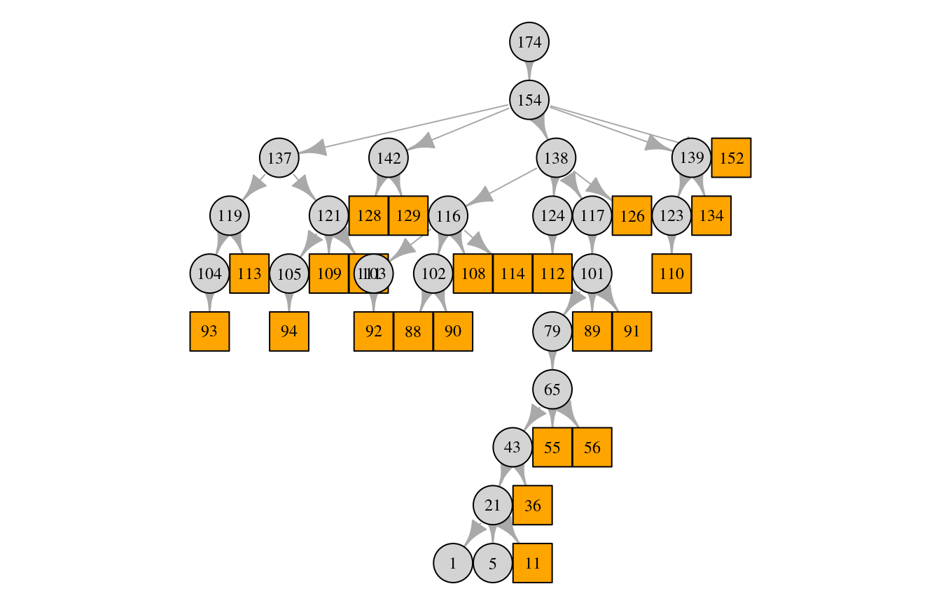
The squares are males and the circles are females.
Adding mitogenomes
We are now ready to add haplotypes/mitogenomes to the individuals. Let us consider
sites <- 100in the mitogenome for know.
First, we construct a function to create founder haplotypes. Here, they are just random:
get_founder_mito <- function() {
  sample(c(FALSE, TRUE), sites, replace = TRUE)
}
x <- get_founder_mito()
head(x)
## [1] TRUE TRUE TRUE FALSE FALSE TRUEsum(x)## [1] 51Let us assume the following mutation rates per site:
mu <- rep(1e-2, sites)Now, we can add mitogenomes:
pedigrees_all_populate_haplotypes_custom_founders(
  pedigrees = peds,
  mutation_rates = mu,
  get_founder_haplotype = get_founder_mito,
  progress = FALSE)
We can then try to plot the same pedigree again, this time with information about the individuals’ mitogenomes (namely, the number of variants in each individuals mitogenome):
plot(ped, num_vars = TRUE)
Plotting with the igraph plot quickly becomes difficult to customise. Therefore extensions to the tidygraph/ggraph packages is provided (requires installation of the ggraph package):
if (require("ggraph", quietly = TRUE)) {
  library(tidygraph)
  library(ggraph)

  g <- as_tbl_graph(peds) %>%
    activate(nodes) %>%
    filter(ped_id == ped_id_endgen) %>%
    mutate(num_vars = sapply(haplotype, sum))

  p <- ggraph(g, layout = 'tree') +
    geom_edge_link() +
    geom_node_point(aes(color = sex, fill = num_vars, shape = sex), size = 12, stroke = 2) +
    geom_node_text(aes(label = paste0(name, "\n", num_vars)), size = 4, color = "white") +
    theme_graph(base_family = "") +
    scale_shape_manual(NULL, values = c("Female" = 21, "Male" = 22)) +
    scale_color_manual(NULL, values = c("Female" = "black", "Male" = "red"))
  p
} else {
  cat("The `ggraph` package is not installed, so the figure is not shown.")
}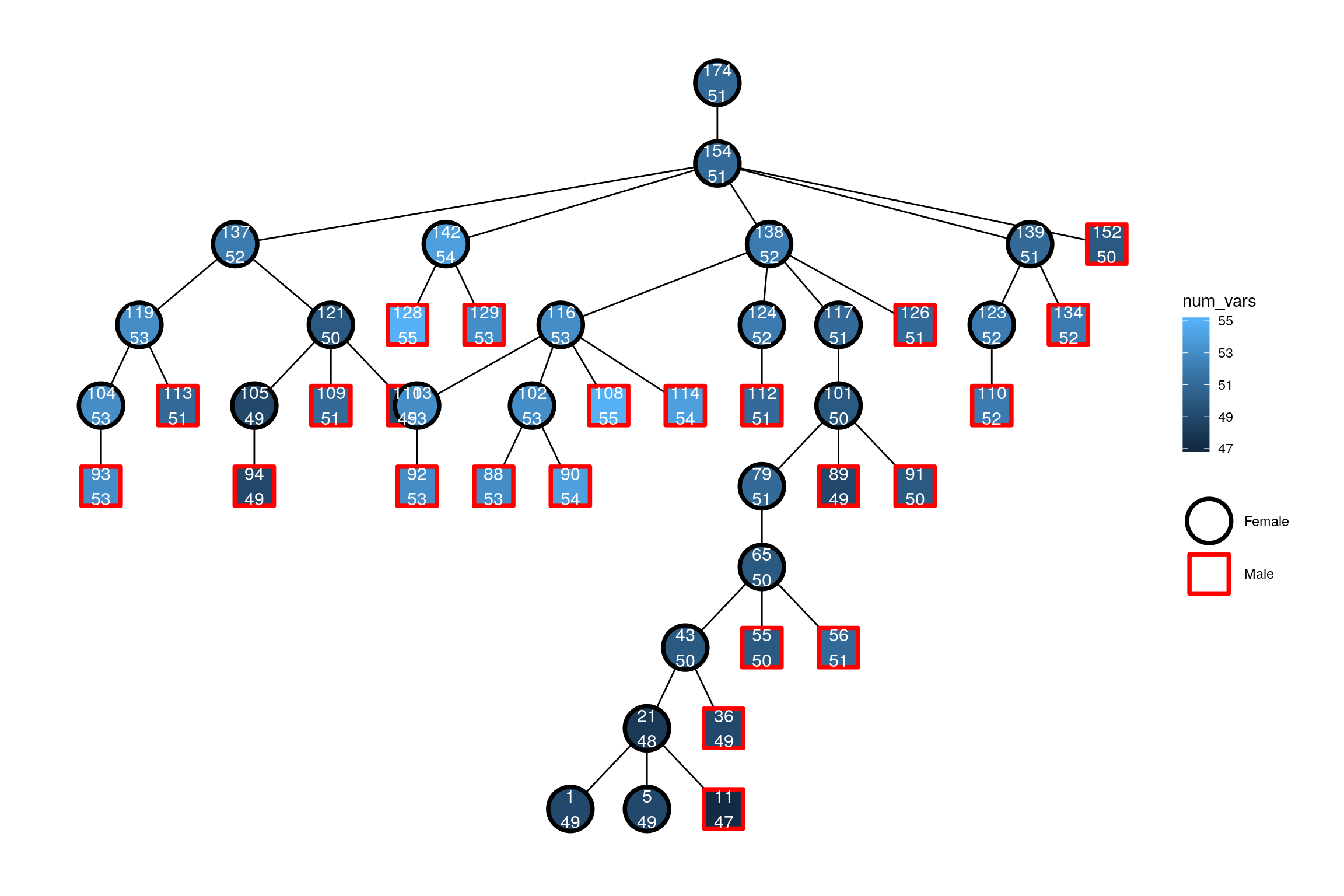
Here, the top number is the id and the number below is the number of variants in the individual’s mitogenome. Note, how it is possible to get both a (border) color and fill for pch values 21-25.
We can also extract all haplotypes in this pedigree:
haps <- get_haplotypes_in_pedigree(ped)
length(haps)
## [1] 46## [1] 51.28261Or from the last male generation by
haps <- get_haplotypes_individuals(sim$end_generation_male_individuals)
length(haps)
## [1] 1000In the simulation function sample_mtdna_geneology_varying_size, there is a parameter generations_return to decide how many generations are returned in the male_individuals_generations and female_individuals_generations elements. The default is 3, meaning that individuals in 3 last generations are returned. So, with the default, the last three generations of males are available in the male_individuals_generations element.
haps <- get_haplotypes_individuals(sim$male_individuals_generations)
length(haps)
## [1] 3000mtDNA mutation schemes
There are several datasets with information about the mitogenome included. There is a help file to each of the datasets which can be found by e.g. ?mtdna_partitions for the mtdna_partitions dataset.
First, there is information about the positions from PhyloTree http://www.phylotree.org/resources/rCRS_annotated.htm about the revised Cambridge Reference Sequence (rCRS) (Andrews et al. 1999):
## # A tibble: 16,569 x 5
##   Position rCRS  PartitionPhyloTree PartitionRieux PartitionOversti
##      <int> <chr> <chr>              <chr>          <chr>
## 1        1 G     Control_region     HVS1 + HVS2    HVS1 + HVS2
## 2        2 A     Control_region     HVS1 + HVS2    HVS1 + HVS2
## # … with 1.657e+04 more rows
Note, that PartitionRieux and PartitionOversti have been modified to obtain the same number of positions as were given in the papers (Rieux et al. 2014; Översti et al. 2017).
There is also mutation information from (Rieux et al. 2014)
data(mtdna_mut_Rieux)
mtdna_mut_Rieux
## # A tibble: 5 x 6
## PartitionRieux MutRateYearly MutHPDLower MutHPDUpper MutRateSEYearly
## <chr> <dbl> <dbl> <dbl> <dbl>
## 1 PC1 + PC2 0.00000000756 5.71e-9 9.35e-9 0.000000000929
## 2 PC3 0.0000000332 2.57e-8 4.07e-8 0.00000000384
## 3 HVS1 + HVS2 0.000000314 2.26e-7 4.03e-7 0.0000000453
## 4 rRNA + tRNA 0.0000000101 7.57e-9 1.27e-8 0.00000000130
## 5 [Not included… 0 0. 0. 0
## # … with 1 more variable: MutationScheme <chr>And from (Översti et al. 2017):
data(mtdna_mut_Oversti)
mtdna_mut_Oversti
## # A tibble: 5 x 6
## PartitionOversti MutRateYearly MutHPDLower MutHPDUpper MutRateSEYearly
## <chr> <dbl> <dbl> <dbl> <dbl>
## 1 PC1 + PC2 0.000000018 1.17e-8 2.40e-8 0.00000000314
## 2 PC3 0.0000000304 1.92e-8 4.21e-8 0.00000000584
## 3 HVS1 + HVS2 0.000000206 1.25e-7 2.90e-7 0.0000000421
## 4 rRNA + tRNA 0.0000000158 9.40e-9 2.30e-8 0.00000000347
## 5 [Not included?] 0 0. 0. 0
## # … with 1 more variable: MutationScheme <chr>Note, that MutRateSEYearly is found by assuming that the HPD (highest posterior density) is a 95% interval from the Normal distribution.
To use the mutation rates from for example mtdna_mut_Rieux:
mu_mean_year <- mtdna_partitions %>%
  left_join(mtdna_mut_Rieux, by = "PartitionRieux") %>% pull(MutRateYearly)
mu_mean_gen <- 25*mu_mean_year
Now, mu_mean_gen contains a mutation rate per generation (of 25 years) for each of the 16569 sites. The probability of one ore more mutations in a single meiosis is then
1 - prod(1 - mu_mean_gen)## [1] 0.01100575Note, that to include variability in the mutation rates, it is probably best to sample a rate per region (in mtdna_mut_Rieux), and then distribute that to all sites in the partition:
d_mu_sample <- mtdna_mut_Rieux %>%
  rowwise() %>%
  mutate(mu = 25*rnorm(1, mean = MutRateYearly, sd = MutRateSEYearly))

mu_sample <- mtdna_partitions %>%
  left_join(d_mu_sample, by = "PartitionRieux") %>% pull(mu)
We can get an impression of the variability of the overall mutation rate:
get_overall_mu <- function() {
  d_mu_sample <- mtdna_mut_Rieux %>%
    rowwise() %>%
    mutate(mu = 25*rnorm(1, mean = MutRateYearly, sd = MutRateSEYearly))

  mu_sample <- mtdna_partitions %>%
    left_join(d_mu_sample, by = "PartitionRieux") %>% pull(mu)

  1 - prod(1 - mu_sample)
}

set.seed(10)
mu_overall <- replicate(100, get_overall_mu())

summary(mu_overall)
## Min. 1st Qu. Median Mean 3rd Qu. Max.
## 0.008937 0.010293 0.010951 0.010940 0.011548 0.013092mean(mu_overall)## [1] 0.0109402## [1] 0.001807331## 2.5% 97.5%
## 0.009229627 0.012720267These rates are easily used to populate mitogenomes:
get_founder_mito <- function() {
  sample(c(FALSE, TRUE), length(mu_mean_gen), replace = TRUE)
}

pedigrees_all_populate_haplotypes_custom_founders(
  pedigrees = peds,
  mutation_rates = mu_mean_gen,
  get_founder_haplotype = get_founder_mito,
  progress = FALSE)
Number of variants in the last three male generations (not just in the one pedigree, but in entire population):
haps <- get_haplotypes_individuals(sim$male_individuals_generations)
table(sapply(haps, sum))
##
## 0 1
## 250042 247028Number of variants in the last male generation (not just in the one pedigree, but in entire population):
haps <- get_haplotypes_individuals(sim$end_generation_male_individuals)
table(sapply(haps, sum))
##
## 0 1
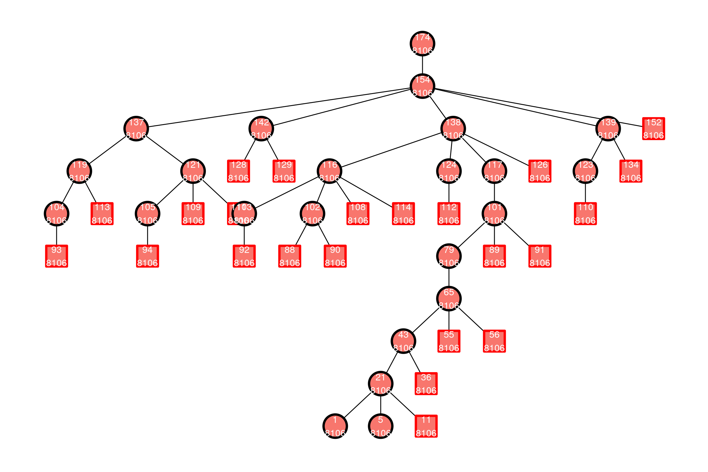
## 83298 82392And the same pedigree with new mitogenomes, now where number of variants is a factor to get a discrete fill colour scale:
if (require("ggraph", quietly = TRUE)) {
  g <- as_tbl_graph(peds) %>%
    activate(nodes) %>%
    filter(ped_id == ped_id_endgen) %>%
    mutate(num_vars = sapply(haplotype, sum))

  p <- ggraph(g, layout = 'tree') +
    geom_edge_link() +
    geom_node_point(aes(color = sex, fill = factor(num_vars), shape = sex), size = 12, stroke = 2, show.legend = FALSE) +
    geom_node_text(aes(label = paste0(name, "\n", num_vars)), size = 4, color = "white") +
    theme_graph(base_family = "") +
    scale_shape_manual(NULL, values = c("Female" = 21, "Male" = 22)) +
    scale_color_manual(NULL, values = c("Female" = "black", "Male" = "red"))
  p
} else {
  cat("The `ggraph` package is not installed, so the figure is not shown.")
}
References
Andersen, MM, and DJ Balding. 2017. “How convincing is a matching Y-chromosome profile?” PLOS Genetics 13 (11): e1007028.
Andrews, Richard M, Iwona Kubacka, Patrick F Chinnery, Robert N Lightowlers, Douglass M Turnbull, and Neil Howell. 1999. “Reanalysis and revision of the Cambridge reference sequence for human mitochondrial DNA.” Nature Genetics 23.
Översti, Sanni, Päivi Onkamo, Monika Stoljarova, Bruce Budowle, Antti Sajantila, and Jukka U. Palo. 2017. “Identification and analysis of mtDNA genomes attributed to Finns reveal long-stagnant demographic trends obscured in the total diversity.” Scientific Reports 7.
Rieux, Adrien, Anders Eriksson, Mingkun Li, Benjamin Sobkowiak, Lucy A. Weinert, Vera Warmuth, Andres Ruiz-Linares, Andrea Manica, and François Balloux. 2014. “Improved Calibration of the Human Mitochondrial Clock Using Ancient Genomes.” Molecular Biology and Evolution 31 (10): 2780–92.