Introduction

library(wgsLR)
library(kableExtra)

Estimating the genotype error probability, $w$

A simple example:

cases <- sample_data_Hp_w(n = 1000, w = 0.1, p = c(0.25, 0.25, 0.5))
tab <- table(cases$xT, cases$xR)
tab
#>    
#>       0   1   2
#>   0 180  53   7
#>   1  55 193  99
#>   2   8  78 327

Maximum likelihood estimation

w_mle <- wgsLR::estimate_w(tab)
w_mle
#> [1] 0.0952511
w_mle_se <- wgsLR::estimate_w_se(tab, w_mle)
w_mle_se
#> [1] 0.005846342

The last lines estimate the standard error that will be used below to construct an approximate confidence interval.

Please be aware of the “Cautionary note” in the README (about not just using standard VCF-files).

Bayesian inference

The package contains a simple Metropolis-Hastings sampler (also see the “Using Stan for Bayesian inference” vignette):

w_b <- wgsLR::estimate_w_bayesian(tab) |> posterior_samples()
w_b_q <- quantile(w_b, c(0.025, 0.975))

hist(w_b, main = NULL, xlab = expression(hat(w)))
abline(v = mean(w_b), col = "deeppink3", lwd = 3)
abline(v = w_b_q[1], col = "deeppink3", lty = 2)
abline(v = w_b_q[2], col = "deeppink3", lty = 2)
abline(v = w_mle, col = "yellow3", lwd = 3)
abline(v = w_mle - 2*w_mle_se, col = "yellow3", lty = 2)
abline(v = w_mle + 2*w_mle_se, col = "yellow3", lty = 2)
legend("topright", col = c("deeppink3", "yellow3"), legend = c("Bayesian", "MLE"), lty = 1, lwd = 2)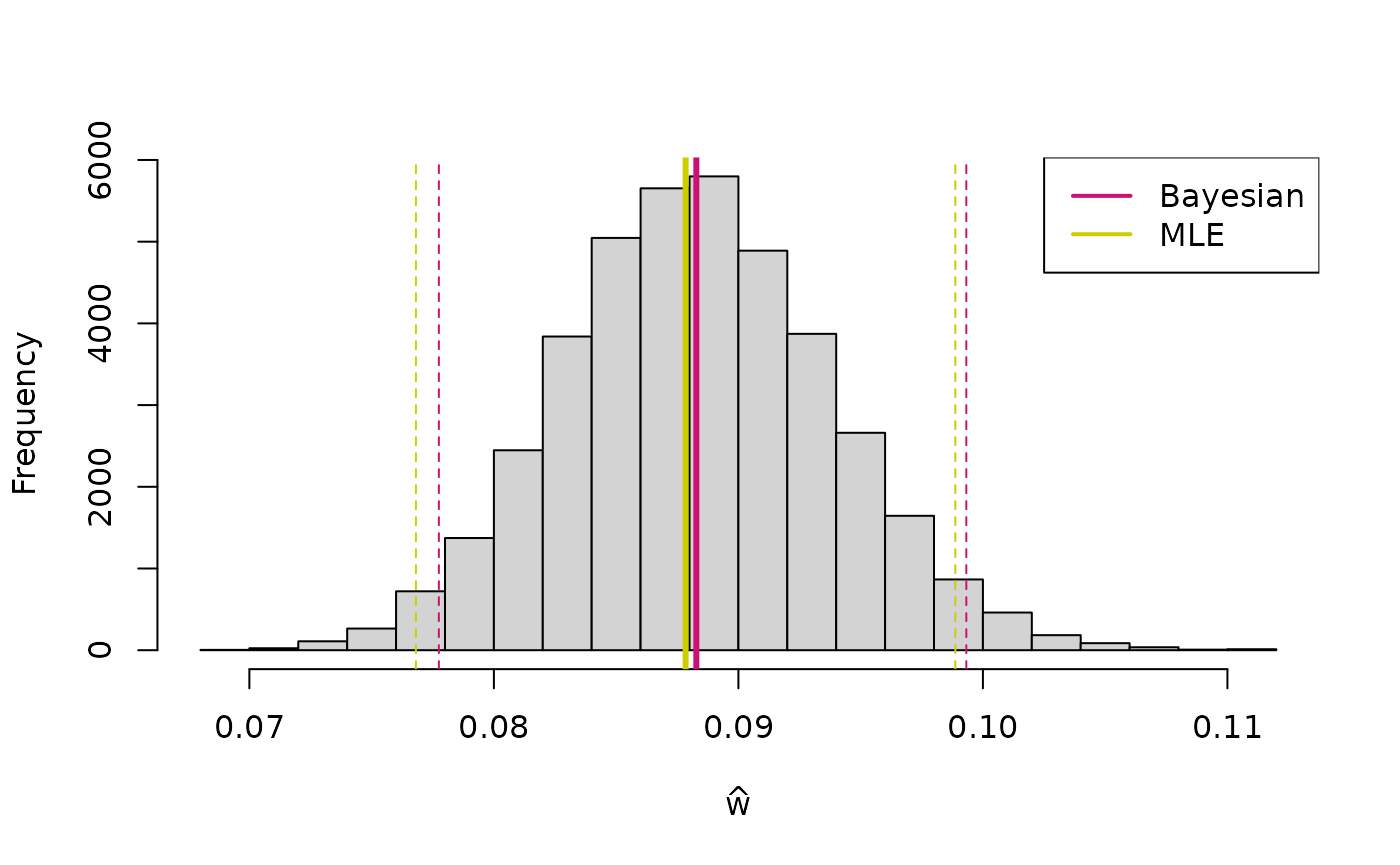

The dashed lines indicate approximate confidence intervals (maximum likelihood estimation) and credible interval (Bayesian inference).

Please be aware of the “Cautionary note” in the README (about not just using standard VCF-files).

Calculating likelihood ratios ($LR$’s)

No errors and matching genotypes:

LR_contribs <- wgsLR::calc_LRs_w(xT = c(0, 0), 
                                 xR = c(0, 0), 
                                 w = 0, 
                                 p = c(0.25, 0.25, 0.5))
prod(LR_contribs)
#> [1] 16

No errors and non-matching genotypes:

LR_contribs <- wgsLR::calc_LRs_w(xT = c(1, 0), 
                                 xR = c(0, 0), 
                                 w = 0, 
                                 p = c(0.25, 0.25, 0.5))
prod(LR_contribs)
#> [1] 0

Errors possible and matching genotypes:

LR_contribs <- wgsLR::calc_LRs_w(xT = c(0, 0), 
                                 xR = c(0, 0), 
                                 w = 0.001, 
                                 p = c(0.25, 0.25, 0.5))
prod(LR_contribs)
#> [1] 15.936

Errors possible and non-matching genotypes:

LR_contribs <- wgsLR::calc_LRs_w(xT = c(1, 0), 
                                 xR = c(0, 0), 
                                 w = 0.001, 
                                 p = c(0.25, 0.25, 0.5))
prod(LR_contribs)
#> [1] 0.04761785

Different error rates

Assume that the trace donor profile has $w_t = 10^{-4}$ and the suspect reference profile has $w_r = 10^{-8}$. Then the $LR$ is:

LR_contribs <- wgsLR::calc_LRs_wTwR(xT = c(1, 0), 
                                    xR = c(0, 0), 
                                    wT = 1e-4, 
                                    wR = 1e-8,
                                    p = c(0.25, 0.25, 0.5))
prod(LR_contribs)
#> [1] 0.003198241

Verifying formulas

The usual $LR$ values, $\frac{1}{p_{Z^S}}$ for matches and $0$ for non-matches, are obtained when setting $w = 0$. For example with both packages wgsLR and caracas loaded we can do the following:

library(caracas)
LR <- d_LR_w$expr
LRw0 <- sapply(LR, \(x) as_sym(x) |> subs("w", 0) |> as_character())
with(d_LR_w, cbind(xT, xR, LRw0))
#>       xT  xR  LRw0   
#>  [1,] "0" "0" "1/p_0"
#>  [2,] "0" "1" "0"    
#>  [3,] "0" "2" "0"    
#>  [4,] "1" "0" "0"    
#>  [5,] "1" "1" "1/p_1"
#>  [6,] "1" "2" "0"    
#>  [7,] "2" "0" "0"    
#>  [8,] "2" "1" "0"    
#>  [9,] "2" "2" "1/p_2"

And with sample specific error rates, $w_D$ and $w_S$:

library(caracas)
LR <- d_LR_wTwR$expr
LRw0 <- sapply(LR, \(x) as_sym(x) |> 
                 subs("wT", 0) |> 
                 subs("wR", 0) |> as_character())
with(d_LR_wTwR, cbind(xT, xR, LRw0))
#>       xT  xR  LRw0   
#>  [1,] "0" "0" "1/p_0"
#>  [2,] "0" "1" "0"    
#>  [3,] "0" "2" "0"    
#>  [4,] "1" "0" "0"    
#>  [5,] "1" "1" "1/p_1"
#>  [6,] "1" "2" "0"    
#>  [7,] "2" "0" "0"    
#>  [8,] "2" "1" "0"    
#>  [9,] "2" "2" "1/p_2"